Microarray Image Processing.

 

Image processing is done with the Xplore program. Input for this program are arrays images produced by scanner and annotation file produced by the spotter. The Xplore output is a file containing values of integral fluorescence of the surface of the microarrays carrying the DNA spots. Besides this the Xplore offers a number of tools for visual and statistical analysis of the substrate surface.

 

Image Loading.

 

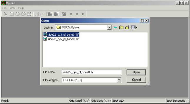
Selection of the FileàOpen menu item opens the standard file open dialogue. The dialogue shows files with TIFF extension because only that standard supported by the Xplore. Select desired file and press the <Open> button.

 

 

After the file is opened the Xplore main window looks in the following way:

 

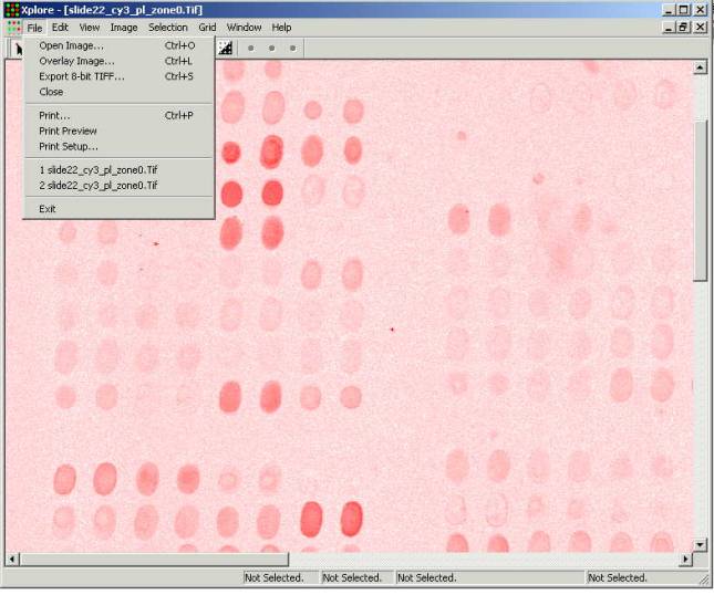
Image of the first opened image is being drawn by the red color. (Please note that a microarray of rater low quality has been selected for this manual in order to demonstrate all advantages of the Xplore. The microarray selected contains printing, processing and scanning defects yet it is still possible to extract meaningful data out of this experiment.)

 

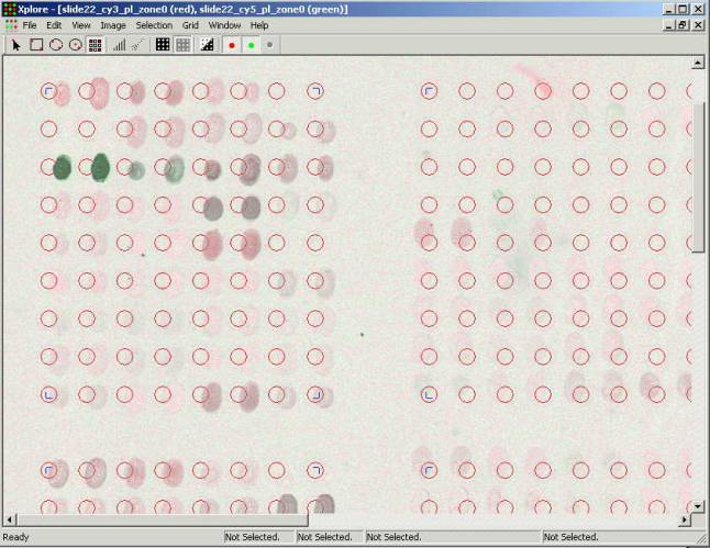
Composite Image.

 

When the first image was opened a few additional items were added to the Fileà… menu.

 

 - Overlay Image - allows overlaying another images made in the other scanner channels over the one that has already opened.

- Export 8-bit TIFF - allows to save the image in the 8 bit TIFF format that is compatible with the majority of commercial graphical software. This file is intended for the purposes of presentations and publication of experimental materials and does not contain any quantitative information.

 

Selecting the FileàOverlay Image opens the same file open dialogue. It is important to open only images of the same microarray obtained in the other scanning channels for overlaying. Otherwise the program reports an error and prevents the incorrect image from being overlaid over the first one. If the image overlay operation went successfully the Xplore window starts looking in the following way:

 

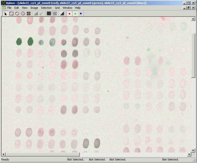
The second opened image is being drawn with the green color. The Xplore allows three images to be overlaid. The third overlaid image will be in the blue color. (All examples in this manual were prepared using two images obtained by scanning a microarray in the channels that correspond to Cy3 and Сy5 fluorescent dyes).  Pressing buttons with colored dot at the toolbar turns on and off corresponding images. When all buttons are pressed the images are overlaid forming the composite image. When images overlay the colors mix proportionally to the intensity of the surface elements (pixels). If intensity is equal in both channels this area is being shown gray. Intensity level of the gray color corresponds to the level of intensity of the surface.  Prevailing of the red or green color indicates the difference of fluorescence intensity in the channels.  Color intensity is proportional to the fluorescence intensity in the corresponding channel. It is correct to assume that colored spots carry clones that expressed differently in this experiment and the gray ones have no differential expression.

 

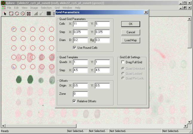
Applying the Grid.

 

The grid defines zones of data extraction. In order to perform proper data extraction it is necessary to place the grid cells over the corresponding spots on the images.

Go to GridàDefine Grid menu item to open the Grid Parameters dialogue.

 

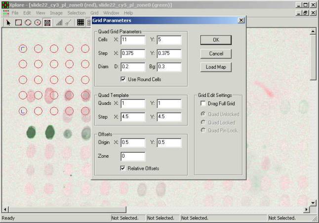
It is possible to define grid manually or load a file with microarray layout generated by the spotter. A grid done manually does not contain annotation of the clones, while the grid that is taken form the generated file contains both annotation of clones on the chip and their positions.

In order to load a file with grid parameters generated by the spotter press the <Load Map> button in the Grid Parameters dialogue window. At the standard file open dialog select the appropriate file. The Xplore main window after the grid has been applied shown below:

 

Grid cells approximately fit positions of the spots. The objective of the further operations with the grid is to place the cells exactly over the spots. Average time requires to position the grid over a 1000 clones array is about 10 minutes, however for larger array of a number thousands spots this may take a significant time.  In order to make interruptions in this continuous process saving intermediate parts of the work it is possible to save edited grid in a file. To do this select the GridàSave Grid menu item. The grid will be saved in a file with .grd extension. In order to get back to the same image open the saved grid file not the one that was originally produced by the spotter.

 

Manual Grid Adjustments.

 

The Xplore does not allow moving each cell individually. That would have been too laborious indeed. There are alternative means built in the program that allow adjusting the grid fast and accurately.

In order to move all cells of the grid simultaneously move the pointer to a blue angle in one of the corners of the quads of spots in the array. Holding the <Shift> button at the keyboard and the left button of the mouse move the entire quad of the grid cells all the way to combine the left upper cell of the grid with the left upper spot in the array.

 

 

After that select the GridàDefine Grid menu item and in the opened window "Grid Parameters" press the <OK> button doing no other actions. This will result in shifting of all of the grid cells at the same distance and in the same direction as the first quad did. If there are no printing defects at the chip this may be the last step required to combine the grid cells with the corresponding spots. However if the microarray has been printed with some quads off the rectangular formation it is necessary to process each of the quads individually.

It is possible to distort the rectangular form of the grid if it's necessary to reflect some distortions of the pattern the spots have printed. Left click on a one of the blue angles in the quads corners and drag it without holding the <Shift> key. The grid cells will move as if they attached to a rubber thread.

 

That is the way of dealing with distortions inside a quad. For the vast majority of images this procedure is enough to place all cells accurately over the spots and proceed to the data extraction.

 

Automated Grid Adjustment.

 

In case of major printing defects it is possible to apply one of the automated algorithms that designed to locate spots and move each of the cells individually. In order to do this it is necessary to perform all above actions and place the grid manually with the maximal possible accuracy. After that select one of the menu items: GridàAdjust Grid 2DW or GridàAdjust Grid 1DW or GridàAdjust Grid CM. The program place grid cells in the areas of the maximum intensity. Use the algorithm that brings the best results for a particular image/

 

 

Please note that due to independent movements of the grid cells some of the cells can be placed significantly asymmetrically.

 

Data Extraction Zones.

The process of data extraction deals with integrating of intensity all pixels circumscribed by the grid cells borders for each of the scanning channels apart and saving the integral intensity values in a file that can be used by the data analysis software.

There are zones of integration of the intensity take place during the data extraction - the SIGNAL zone and the BACKGROUND zone. Knowledge of the background level around spots gives indirect information regarding quality of the experiment. Each of the cells drawn as two concentric circles: red and blue. These circles limit the signal and the noise zones correspondingly for a particular cell. The ring between the circles is a border zone. No data extracted out of it.

 

 

 

 

 

 

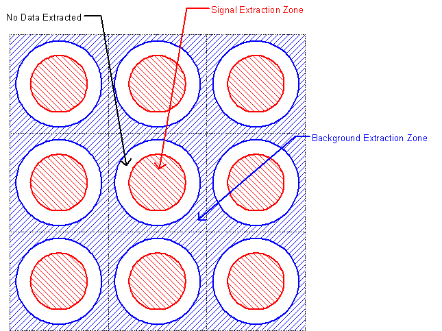
The default signal zone diameter is equal to the diameter of the printing needles used for this microarray. The default background zone diameter is 1.5 times bigger. It is possible to change those parameters manually. To do so open the Grid Parameters dialogue following the GridàDefine Grid menu item.

 

 

Data fields next to the "Diam." label define diameters of the zones "D:" of the signal and "Bg:" of the background. The rest of the fields in this dialogue mean following:

Quad Grid Parameters

- Cells X: Y: number of grid cells along the X and Y axes.

- Step X: Y: distance between cells along the X and Y axes.

- Use Round Cells option of using round cells vs. squared ones. (in case of the squared cells diameter means side of the square)

 

Quad Template

- Quads X: Y: number of spot quads along the X and Y axes.

- Step X: Y: distance between quads (typically equal to the distance between the needles)

 

Offsets:

- Origin X: Y: position of the low left spot on the chip relative to the low left corner of the substrate.

- Zone - printing zone number in case of multiple zones.

- Relative Offsets - adds zone offset specified in slide description file produced by printer program.

 

 

 

 

To extract the data select the GridàExtract Grid Data menu item. In the opened standard file saving dialog type the name of the integral intensity data file and press the <Save> button. This file has can be used by the Xplain data processing program or by a third party software such as Excel or Mathlab.

 

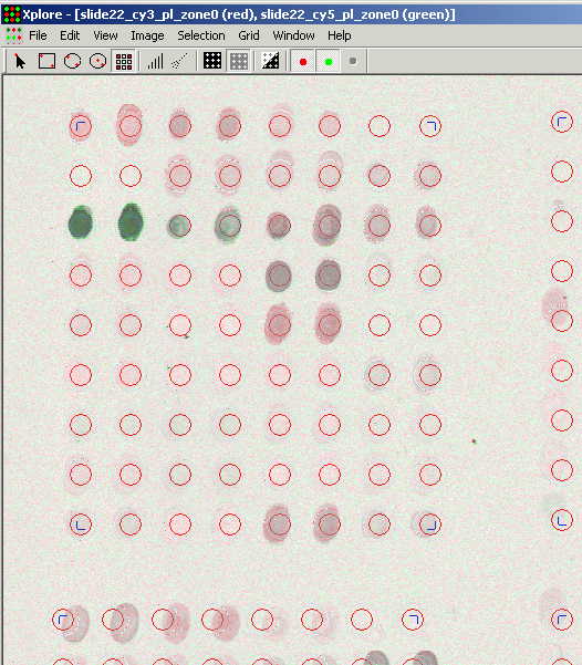
Clones Search.

 

Combination of the <Ctrl> and <F> at the keyboard opens the search window.

 

 

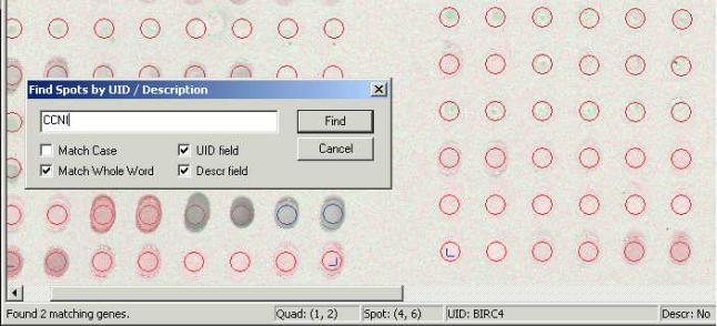
Enter the name of the clone or a part of the name in the search field. If the exact name is known mark the "Match Whole Word" checkbox, otherwise mark the "Match Case" checkbox. The other two checkboxes in the dialog window define the fields the desired annotation will be searched in. Search results shown in the left side of the status bar indicating the number of occurrences found in the search. All the corresponding cells are being highlighted in the same time with the blue circle. (The circle line is single width compare to manual selection).  In the example shown at the picture above two clones were found which is witnessed by the "Found 2 matching genes" message. The spots have found located in the middle of the second row from the bottom.

 

 

 

Location of Low Intensity Spots.

 

It is typical to deal with low intensity images in the most of the microarrays experiments. Signal to Background (S/B) ratio of low intensity spots is less than 10. However even spots with signal to background ration around 5 may bring reliable information. Spots with such a S/B ratio can be barely recognized on the image. It might be difficult to locate them and place the grid correctly. The Xplore provides certain tools to locate the low intensity spots.

 

Image Inversion.

 

The   button inverses the image.

 

 

In some instances low intensity spots appear more contrast on dark background. Inversion changes the picture only and does not affect the data.

 

Background Subtraction

 

One of the  buttons starts the selection mode. The shape of the zone is being selected corresponds to the picture at a particular button. It is necessary to select a background area between the spots and go to the ImageàSubtract Background menu item. From intensity of each pixel the program will subtract average intensity of the selected zone. The image will become lighter (darker in the inverse mode) and this may result in increase in contrast.

 

Statistical Analysis.

 

The "Xplore" offers means for basic statistical analysis of the selected zone. Pressing the  button (or selecting the SelectionàShow Selection Statistics menu item) opens the Selected Data Statistics dialog:

 

 

 

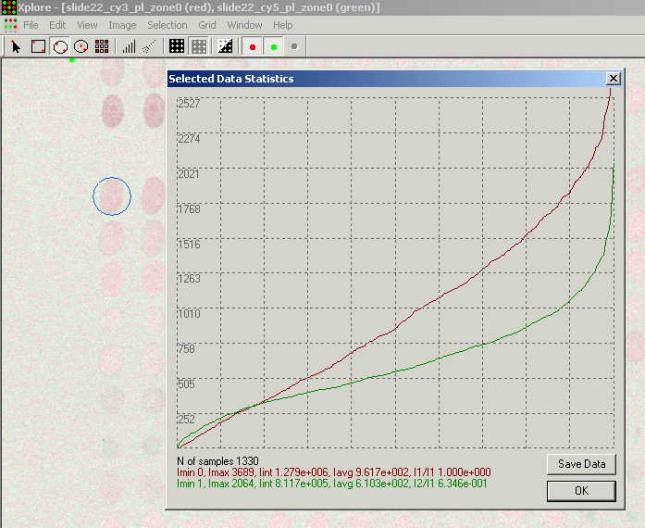
In the upper part of the opened window shown the histogram of intensity of the pixels from the selected zone for each of the scanning channels. The X axis shows number of pixels of a particular intensity. The Y axis shows pixels intensity in the dynamic range of the current selection zone. The red line represents data for the first opened channel the green one for the second channel.

 

In the bottom part of the window basic statistics is shown:

 

N of samples: 1330 - means that the selected area contains 1330 pixels.

I min 0 - minimal intensity pixel has intensity equal to 0 (1 for the green channel)

Imax. - maximal intensity pixel

Iint. - integral intensity for all pixels in the selected area

Iavg. - average intensity for all pixels in the selected area

I1/I1 ( I1/I2 )- ratio of integral intensities of the pixels from two channels. Meaningless for one opened channel - equal 1. If two channels are open - it is I1/I2; equal to 0.6346 in this example.

Histogram data can be saved in a txt file by pressing the <Save Data> button.

 

Equalizing Sensitivity of Scanner Channels.

 

Due to the non-uniform labeling of hybridization probes fluorescent levels of Cy3 and Cy5 dies may differ significantly. It is important to adjust sensitivity of scanner channels to obtain images with approximately equal average values of the intensity. We recommend using the dialog described in the previous paragraph to obtain data of the average intensity (Iavg.) for both channels. Select a large area of the image that covers both background zone and the zone where spots reside. If average intensity values of two channels of the area selected differ more than 10-15% from each other try to decrease sensitivity of the channel with the higher intensity. Rescan the microarray with the new sensitivity settings. Repeat measurements and rescanning till the both channels of the scanner produce images with equal Iavg. values.

 

Scatter plot.

 

Pressing the  button opens the Selected Data Pairs dialog.

 

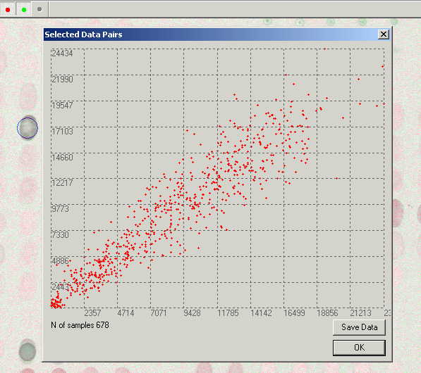
The X and Y axes show value of intensity in the first and the second channels correspondingly. Spots at the chart indicate intensities of pixels from the selected area.